
N3Sim Project
User Guide
Overview
N3Sim is a simulation framework for diffusion-based molecular communication in nanonetworks, a bio-inspired paradigm
based on the use of
molecules to encode and transmit information.
N3Sim simulates a set of nanomachines which communicate through molecular diffusion in a fluid medium. The information to be sent by the emitter nanomachines modulates the rate at which they release particles to the medium. The variation in the local concentration generated by the emitters propagates throughout the medium. The receivers are able to estimate the concentration of particles in their neighborhood by counting the number of particles in the environment. From this measurement, they can decode the transmitted information.
This is the user guide for the version 0.7 of N3Sim. It includes a general description of the simulator in sections Current Features and N3Sim Block Diagram. Installation and execution instructions may be found in sections Installation, Running Simulations, Output and Automating Simulations. Finally, more specific concepts about the simulator are explained in the remaining sections.Contents
- Current Features
- Roadmap
- N3Sim Block Diagram
- Installation
- Running Simulations
- Output
- Automating Simulations
- 3-Dimensional Simulations
- Time and Time step
- Anomalous Diffusion Components
- Simulation Space
- Simulating an Infinite Space
- Emitters
- Receivers
Current Features
N3Sim is a prototype still under development. Some of its features are therefore under testing and are not available in the current released version (v0.7). For instance, the influence of electrostatic forces in diffusion is not included in v0.7, and 3-dimensional simulations are only possible when the particles move according to Brownian motion in an unbounded space.
The current features of N3Sim are:
- Brownian motion and components of anomalous diffusion: particle inertia and ellastic collisions for 2-dimensional space. (A prototype that includes the electrostatic forces among particles is currently under testing.)
- All components of diffusion can be activated/deactivated.
- Bounded or unbounded space.
- Initial background homogenous concentration (finite or infinite space).
- Any number of emitters and receivers.
- Predefined released patterns for each emitter.
- Input file (.txt) defined by the user containing a released pattern for each emitter.
- 3-dimensional simulation (only for Brownian motion an unbounded space).
Roadmap
The current stable version of N3Sim is v0.7. Some of the new features that will be included in next versions are:
- v0.8: electric forces as a component of anomalous diffusion.
- v0.9: obstacles in the simulation space.
- v1.0: complete 3-dimensional simulations.
N3Sim Block Diagram
Figure 1 shows a block diagram of the steps needed to run a simulation.
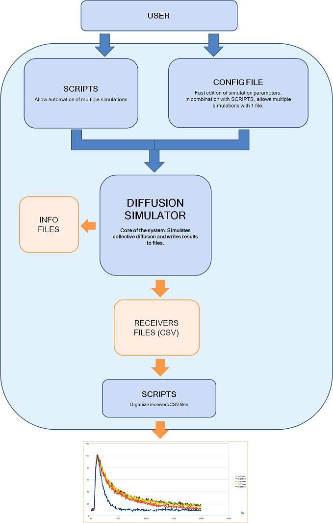
Figure 1. N3Sim block diagram
First, the user communicates with the simulator using a configuration file and, optionally, a script. In the configuration file, the user specifies the values of all the simulation parameters. These parameters include the number and location of emitters and receivers, the waveform of the emitter, the size of the emitted particles and the diffusion coefficient of the medium, amongst others. Some of this parameters can be left unspecified and can be defined using an script; this allows the user to run multiple simulations automatically with only one configuration file an one script. This is useful to easily evaluate the influence of a specific parameter (e.g., the number of transmitted particles) in the system output.
Next, the diffusion simulator takes the configuration file and the automation scripts as input and performs the actual simulation. The diffusion simulator writes its results to files. To do so, it creates a new folder with the simulation name and in this folder creates one file per receiver and some other files with the simulation information. The receiver files are text files in csv format, they contain the concentration measured by each receiver as a function of time. Last, another set of scripts may be used to organize the results from several receivers and graphically represent them into a single plot.
Installation
N3Sim is a Java runnable jar file. It is OS-independent as long as the Java VM is installed in the system. In order to use N3Sim, Java 1.6 or higher is required. If you do not have Java in your system, you may download it from here.
In order to install N3Sim, just download the executable jar file and the configuration file from here.
Running Simulations
In order to run a simulation with N3Sim, you first need to edit the values of the simulation parameters. To do so, just open the text file N3Sim.cfg previously downloaded, which has all the parameters set to their default values. You may edit them in order to fit your requirements and then save the configuration file with the desired name. A list of parameters together with a brief explanation of them is available here. A more comprehensive explanation of some of the parameters can be found in the following sections of this guide.
Once the configuration file has the desired values, enter the following command in a Unix shell or Windows command prompt from your N3Sim directory::
> java -jar N3Sim-0.7.jar myConfigFile.cfg
For simulations with a high number of particles, you may want to increase the amount of Java memory up to, e.g., 1024M.
> java -jar -Xms1024m -Xmx1024m N3Sim-0.7.jar myConfigFile.cfg
This will start the simulation. Once it is complete, just check its results (see section Output).
Output
Once the simulation has finished, the application will have created a directory under the N3Sim folder with the name specified by the parameter outPath in the configuration file. Inside this folder, the following files may be found:
- A file simulation.txt with the parameters and values used in the simulation.
- A file receiver_name.csv for each receiver in the simulation. These files have two columns; the first one contains the time steps in nanoseconds, and the second one represents the number of particles measured by the receiver at the corresponding time step.
- Debugging files info.log (optional) and error.log.
- Video file graphic.ns1 (optional), to be used with NSVideo.
Automating Simulations
Often user is interested in performing multiple identical simulations in order to compute the average results, or to check how the results change depending on the values of one or more parameters.
N3Sim provides the following mechanism to facilitate the execution of multiple simulations. In the configuration file, one or more parameters can take the key value "param". In this case, the program expects to receive these parameters from the execution command (in the same order that they are in the configuration file.) For instance, if the value "param" is given to the parameters time and timeStep, the simulation may be executed as follows:
> java -jar N3Sim-0.7.jar myConfigFile.cfg 2000 5
which is equivalent to give the values time=2000 and timeStep=5 in the configuration file.
In this way, scripts can be used to launch multiple simulations with different parameters. An example: let's imagine we want to run several 2-dimensional simulations combining different values of particle radius (1, 2, 5 and 10 nm) with several values of diffusion constant D (0.5, 0.6, 0.7, 0.8 and 0.9 nm^2/ns).
By using the word "param" as the value for any parameter, the program will read its value from the parameters list of the execution command (in the same order that they appear in the configuration file).
In this example, we give the value "param" to the parameters outPath (so that each simulation has a different folder), sphereRadius and D, as shown in figure 2. Then, the script shown in figure 3 will run the multiple simulations.
### SIMULATION PARAMS
outPath=param
graphics=false
infoFile=true
activeCollision=false
BMFactor=1
inertiaFactor=0
time=200000
timeStep=1000
### SPACE PARAMS
boundedSpace=true
constantBGConcentration=false
constantBGConcentrationWidth=0
xSize=2500
ySize=2000
D=param
bgConcentration=10
sphereRadius=param
### EMITTER PARAMS
emitters=1
emitterRadius=100
x=1000
y=500
startTime=1000
endTime=2000
initV=0
punctual=false
concentrationEmitter=false
color=white
emitterType=1
amplitude=1000
### RECEIVER PARAMS
receivers=1
name=rx500
x=1500
y=500
absorb=false
accumulate=false
end=true
Figure 2. Configuration file used to launch simulations combining different values of the parameters sphereRadius and D.
#!/bin/sh
# These script will launch simulations combining values of PARAM1_LIST# with values of PARAM2_LIST.
# Simulation results will be stored in folders named "myTest-i-j",
# where i and j are the values of the parameters.
PARAM1_LIST=(1 2 5 10)
PARAM2_LIST=(0.6 0.7 0.8 0.9)
for i in ${PARAM2_LIST[@]}; do
for j in ${PARAM2_LIST[@]}; do
java -jar N3Sim.jar myConfigFile.cfg myTest-${i}-${j} $i $j
done
doneFigure 3. Script to automate simulations combining lists of values of two parameters.
3-Dimensional Simulations
N3Sim was primarily developed for 2-dimensional scenarios. In the current version, 3-dimensional simulations are possible only under the following conditions:
- Unbounded simulation space
- No collisions among the emitted particles
- Emitter type 5 (see section Emitters)
- Receiver type 3 (see section Receivers)
A specific configuration file for 3-dimensional scenarios, N3Sim3D.cfg, is available. Although the general N3Sim configuration file can also be used for 3-dimensional simulations, it is easier to use the specific 3D configuration file. In this file, the parameters have a predefined value that fullfills the above conditions for 3-dimensional simulations (e.g., boundedSpace = false), and the parameters that may be changed by the user are underlined for easier identification. The template configuration file for 3-dimensional simulations may be downloaded here.
Time and Time Step
The total time of the simulation is set with the parameter time. Time is discrete in the simulator, which advances time by steps (time steps). At each time step, emitters release particles, the simulator moves the released particles according the laws of diffusion, and receivers measure the concentration at their location. Both the parameters time and timeStep must be integers and their unit is nanoseconds.
An important question is: which is the best time step for a simulation? In order to answer it, several criteria must be taken into account. First, it must be noticed that the signal measured by receivers will have a resolution of one time step. The user must thus decide which is the maximum time step so that the obtained results are useful.
On the other hand, in general, the higher the time step the shorter the simulation running time. However, there are several other factors which limit the maximum value of the time step, which are detailed as follows.
First, when modeling Brownian motion and/or inertia, if the time step is too large particles may move in a single time step a long distance, compared to the emitter-receiver distance. The mean distance that particles travel in a time step is sqrt(2*DiffusionConstant*timestep), according to the theory of Brownian motion . In order for the simulation to give reasonably correct results, this value should not exceed the 25% of the distance between emitter and receiver (or the minimum distance between an emitter and a receiver, if there is more than one of them).
For simulations that include collisions among particles, it is still true that the longer the time step, the shorter execution time. However, using a longer time step may cause the number of collisions which happen in every time step to rapidly increase. In this cases, using a smaller time step may result in a less memory consuming simulation and faster execution times.
A useful criteria to check whether the time step used is too large is to perform the same simulation with a smaller time step. If the results are not the same, it means that the time step used in the first simulation was too large. The smaller valid time step is of about 0.0001 nanoseconds.
Anomalous Diffusion Components
N3Sim models anomalous diffusion with four components: Brownian motion, particle inertia, collisions among particles and electrostatic forces.
Electrostatic forces are not yet included in the current version. There is a prototype that includes this component of diffusion, but it is still under testing and has not been released yet.
All the other components can be enabled or disabled. Collisions are activated by the parameter activecollisions, which may be found in the configuration file. Brownian motion and particle inertia may be enabled/disabled through the parameters BMFactor and inertiaFactor, respectively.
Brownian motion models the basic diffusion process which causes the random movement of the emitted particles at every time step. Brownian motion is modeled as a Gaussian random parameter with zero mean and whose root mean square displacement in each dimension after a time t is sqrt(2*DiffusionConstant*timestep). N3Sim multiplies this displacement by the parameter BMFactor. Therefore, if BMFactor is zero no Brownian Motion is performed.
The parameter inertiaFactor accounts for the inertia of particles. At every time step, N3Sim adds a displacement equal to the velocity of the previous time step multiplied by this factor. So, as with Brownian motion, if the inertiaFactor is zero, the particles will have no inertia.
Simulation Space
The simulation space contains the particles, emitters and receivers. Particles are modeled as spheres and its radius is set with the parameter sphereRadius.
The simulation space can be bounded or unbounded. This is controlled by the parameter boundedSpace. If it is true, a rectangular bounded space is simulated. The left/bottom corner of the space is (0,0) and the right/top corner is set at the values of parameters xSize and ySize. In this case, the emitted particles rebound at the space limits (even if the parameter activeCollision is set to false).
The simulation space can be filled before the simulation starts with an initial background concentration. This is set with the parameter bgConcentration, which must be an integer. The units of the background concentration are the number of particles per 10000 nm2. If bgConcentration is not zero, the simulation space must be bounded (boundedSpace = true).
Simulating an Infinite Space
When running simulations with a bounded space, an undesired effect may appear. As emitters release particles, the background concentration will increase indefinitely. Figure 4 shows the signal at a receiver for the same simulation with bounded and with unbounded space. With bounded space (blue line) the tail of the signal is higher than with unbounded space (red line), because of the increase in the background concentration over time.
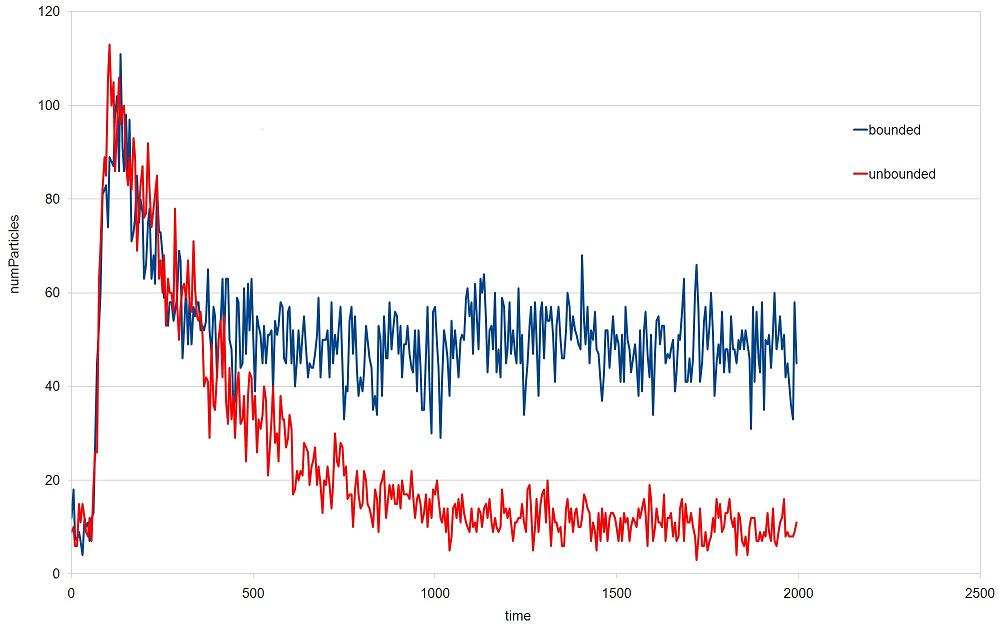
Figure 4. Comparison of a simulation with bounded and with unbounded space.
However, if the initial background concentration is set to a non-zero value, the simulation space must be bounded. In order to avoid this problem, N3Sim offers a mechanism to simulate an infinite space while using a bounded space. This mechanism deletes some particles close to the space bounds, as if they were leaving the space bounds. To activate this mechanism, the parameter constantBgConcentration must be set to true.
A few considerations to be taken into account in order to get the best results follow First, the space dimensions and the proper location of emitters and receivers is crucial. If, for instance, we want to run a simulation with one receiver and one emitter, the distance between the receiver and the space bounds, and between the emitter and the space bounds, must be at least twice the distance between the emitter and the receiver. Otherwise, the simulation of an infinite space will not be realistic.
Second, an important parameter used to adjust this mechanism is constantBGConcentrationWidth. As a rule of thumb, the value of this parameter must be the 2% of the minimum value between the parameters xSize and ySize (see section Simulation Space). If this value is increased, the tail of received signals will be artificially reduced; and if it is decreased, the tail will be increased. In any case, if the size of the space and the location of emitters and receivers have the values indicated in the paragraph above, this parameter has very little influence and the simulation of infinite space is good enough for most cases.
Emitters
The location of an emitter is defined by the parameters x and y in the configuration file. Every emitter has an influence area, which means that the emitter can only release or absorb particles within this area. This area is a circle (or a sphere in 3 dimensions) and its radius is the value of the parameter emitterRadius.
If the emitter tries to emit/absorb more particles than the capacity of its influence area, N3Sim will emit/absorb as many as possible and a message will be written at the error.log file. This message will include the actual number of particles released/absorbed.
Each emitter has an associated waveform that defines the number of particles to be released/absorbed at each time step. Moreover, every emitter has a start time and end time (parameters startTime and endTime). The emitter will emit/absorb particles, according to its waveform, only when the simulation time is greater or equal than startTime and lower than endTime.
There are five types of emitters. Three of them have a predefined waveform, and they have a parameter named amplitude. The amplitude is the number of released particles every 100 ns. For instance, if the time step is of 400 ns and 1000 particles must be released at every time step, the parameter amplitude must be set to a value of 250.
The three emitters with a predefined waveform are:
- Type 1: emits a fixed number of particles at every time step.
- Type 2: emits particles following a rectangular waveform. For this emitter, two additional parameters exist: period and timeOn. These parameters indicate, respectively, the period of the square wave and amound of time within a period in which the emitter is releasing particles (as many as indicated by the parameter amplitude).
- Type 3: emits particles following a white noise waveform.
Type 4 emitters read the waveform of the signal to be transmitted from a text file. In this text file, every line represents a time step, beginning at startTime. At every time step, the number of particles indicated by the corresponding line are emitted. If the total number of lines of the text file is lower than the number of time steps between startTime and endTime, zeros are assumed. The parameter file indicates the filename where the waveform is defined (including relative or absolute path). Another parameter for this emitter is scaleFactor. Emitters multiply the number of particles specified in the file by this factor in order to obtain the number of particles to emit, which is useful to automate simulations.
Finally, Type 5 emitters are equivalent to type 4, but in a 3-dimensional simulation space. For this emitter, the z location must be set using the parameter z in the configuration file.
Receivers
The receive location is defined by the parameters x and y in the configuration file. Receivers count the number of particles in its area (or volume) at every time step. This number is written to the receiver result files (see section Output)
There are three types of receivers. First, Type 1 receivers are square receivers, and their size is defined by the square side (parameter side). Second, Type 2 receivers are circular, their size is defined by their radius (parameter rradius). Last, Type 3 receivers (to be used in 3-dimensional simulations) are spherical receivers and the counting volume is also defined by its radius (parameter rradius).
Receivers may just count the particles inside their area (or volume), or they may also absorb these particles. This is controlled with the parameter absorb. Finally, the accumulate parameter controls whether the receiver output corresponds to the instantaneous particle count ( accumulate=false), or to the accumulated particle count since the beginning of the simulation (accumulate=true).
